Fluorescent Microscopy: The Art and Science Unveiled

Fluorescent microscopy is not a transparent window but a powerful translation; its true “art and science” is the disciplined practice of managing inherent signal ambiguity. The glow you see represents both biological reality and technical artifact—distinguishing between them requires a systematic understanding of the trade-offs.

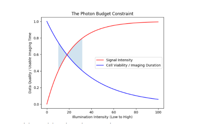
Visualizing the Fundamental Trade-Off: The Photon Budget

Every fluorescent experiment operates under a fundamental constraint: fluorophores emit a finite number of photons before bleaching. How you manage this “photon budget” determines whether you collect meaningful data or artifacts.

The Complete Framework: Science, Art, and Practical Implementation

The following tables systematically break down each component of fluorescent microscopy, moving from core science to practical application.

The Scientific Components & Their Hidden Ambiguities

Component	Primary Function	Key Parameter	Hidden Ambiguity/Caveat	Critical Question to Ask
Fluorophore	Light-emitting molecule	Extinction coefficient, quantum yield	Finite photon budget; photobleaching is irreversible	“Am I maximizing signal through preparation rather than just increasing laser power?”
Excitation Source	Provide excitation light	Intensity, wavelength stability	Phototoxicity: light damages living samples	“Is my observation altering the biology I’m trying to study?”
Optics & Objective	Collect and focus light	Numerical Aperture (NA), magnification	Shallow depth of field creates 2D illusion from 3D reality	“What’s happening above and below my focal plane that I’m missing?”
Filters & Dichroics	Separate excitation from emission	Bandwidth, transmission efficiency	Spectral bleed-through (crosstalk) between channels	“Is my ‘specific’ signal contaminated from other fluorophores?”
Detector (Camera/PMT)	Convert photons to signal	Gain, read noise, quantum efficiency	Gain amplifies noise alongside signal	“Is this dim structure real signal or amplified noise?”
Sample Environment	Biological context	Refractive index, temperature, pH	Autofluorescence creates false positives	“Have I imaged an unlabeled control under identical conditions?”

References & Further Reading: Fluorescent molecules soak up light energy, get excited, and spit it back out at a different wavelength—think absorbing blue and beaming green. The microscope’s the maestro, wielding filters and beams to catch that shift.

The Interpretive “Art” – From Design to Analysis

Process Stage	Common Misconception	Reality (The True “Art”)	Practical Framework	Example Failure Mode
Experimental Design	“Controls are just for publication”	Pre-visualization of all possible artifacts	The Control Matrix: Run autofluorescence, secondary-only, and positive controls in parallel	Mistaking tissue autofluorescence for specific labeling
Sample Preparation	“More label = better signal”	Optimization for specificity over intensity	Titration approach: Find the minimum label concentration that gives a detectable signal above controls	Non-specific binding creating false localization patterns
Image Acquisition	“Maximize all settings for best image”	Strategic trade-off management	The Triangle Constraint: Choose 2: Speed, Resolution, Sensitivity	Photobleaching the entire sample before completing the time series
Live-Cell Imaging	“Just use lower light”	Balancing observation with perturbation	Viability vs. Visibility Index: Establish metrics for cell health during imaging	Documenting stress responses rather than normal physiology
Image Processing	“Processing reveals hidden truth”	Transparent enhancement of existing data	The Process Receipt: Document every adjustment with software and parameters	Creating structures through excessive deconvolution or thresholding
Data Interpretation	“Colocalization = interaction”	Hypothesis generation, not conclusion	The Resolution Reality Check: 200nm separation can appear as colocalization	Claiming protein interactions without biochemical validation

The Ambiguity Audit Framework – A Step-by-Step Checklist

Audit Phase	Specific Questions	Documentation Required	Acceptable Outcome	Red Flag
1. Pre-Acquisition Design	– What are my 3 most likely artifacts? – Have I designed controls for each? – What is my photon budget strategy?	Written experimental protocol with control rationale	Clear mapping of potential artifacts to specific controls	No biological replicates; single control for multiple conditions
2. Acquisition Parameters	– Are my settings reproducible? – Am I in the linear detection range? – Have I minimized observer bias?	Saved instrument settings file; metadata with images	Settings allow reproduction by trained colleague	Gain set above manufacturer’s linear range recommendation
3. Control Validation	– Do controls look as expected? – Is signal-to-noise > 3:1? – Is autofluorescence < 10% of signal?	Images of all controls with same display settings	Controls show expected negative/positive results	Autofluorescence pattern mimics “specific” signal
4. Processing Transparency	– Can I list every adjustment? – Were identical adjustments applied to all compared images? – Does raw data support processed conclusions?	Processing workflow with software name, version, and parameter values	Raw data visible alongside processed version	Adjustments that “create” data not visible in raw image
5. Interpretation Boundaries	– What are 2 alternative explanations? – Does my conclusion respect optical limits? – What further experiment would confirm?	Written interpretation with acknowledged limitations	Conclusions are conservative and suggest next experiments	Claiming molecular interactions from standard resolution images

Application-Specific Guidelines & Trade-Offs

Application	Primary Goal	Optimal Technique	Critical Trade-Off	Common Pitfall	Validation Required
Protein Localization	Subcellular targeting	Widefield or confocal	Resolution vs. throughput	Misinterpreting overexpression artifacts	Biochemical fractionation + orthogonal method
Live-Cell Dynamics	Temporal tracking	Spinning disk confocal or light sheet	Temporal resolution vs. phototoxicity	Observing stress responses instead of physiology	Cell viability assays post-imaging
Super-Resolution	Nanoscale detail	STORM/PALM or STED	Resolution vs. sampling/throughput	Reconstruction artifacts from sparse sampling	Resolution measurement on biological structure
Multicolor Imaging	Interaction or proximity	Spectral imaging or careful filter sets	Number of channels vs. crosstalk	Spectral bleed-through misinterpreted as colocalization	Unmixing controls and spectral validation
Quantitative Intensity	Concentration measurements	Widefield with careful calibration	Signal linearity vs. dynamic range	Ignoring non-linear detector response	Standard curves with known concentrations
Clinical/Diagnostic	Reproducible detection	Standardized widefield	Sensitivity vs. specificity	Inter-operator variability	CLIA-type validation with positive/negative controls

The Evolution of “Art” with Computational Advances

Traditional Skill	Computational Equivalent	New Ambiguity Introduced	Required New “Art” Skill	Quality Control Metric
Manual focus optimization	Automated focus algorithms	Algorithm failure on heterogeneous samples	Understanding algorithm failure modes	Visual verification of focus across field
Visual filter selection	Spectral unmixing	Mathematical solutions not biologically valid	Recognizing physically impossible unmixing results	Validation with single-label controls
Expert thresholding	Machine learning segmentation	Training set bias	Critical evaluation of training data representativeness	Performance on diverse, unseen test images
Judicious deconvolution	AI-based restoration	Hallucination of plausible structures	Distinguishing between restoration and invention	Comparison with physical resolution limits
Qualitative assessment	Quantitative feature extraction	Statistical vs. biological significance	Understanding multiple testing and effect sizes	Power analysis and false discovery rates

Synthesis: The Integrated Practitioner’s Mindset

The tables above reveal that fluorescent microscopy expertise isn’t a linear progression but a simultaneous management of multiple dimensions:

1. The Resource Dimension(Photon budget, time, sample viability)
2. The Artifact Dimension(Autofluorescence, bleed-through, noise)
3. The Interpretation Dimension(Optical limits, statistical significance)
4. The Technological Dimension(Tool capabilities and limitations)

Expert practitioners don’t avoid these constraints—they map them systematically. The “art” is knowing which constraints are flexible for a given biological question and which are absolute boundaries.

Practical Implementation: Your First-Experiment Roadmap

For beginners, follow this prioritized sequence:

1. Week 1-2: Master Controls

• Imagine your sample type without any labels (autofluorescence baseline)
• Optimize fixation/permeabilization to minimize background
• Establish what “zero” actually looks like in your system

2. Week 3-4: Single-Channel Optimization

• Titrate your primary label to find the minimum concentration for detection
• Document the exact relationship between laser power and bleaching rate
• Establish your system’s practical signal-to-noise limits

3.Week 5+: Add Complexity Gradually

• Add the second channel only after the first is fully characterized
• Validate separation empirically, not just from filter specifications
• Always maintain the control disciplines established in Week 1

Conclusion: Beyond the Binary

The “art and science” framework is misleading if seen as separate domains. The science reveals what’s technically possible; the art navigates what’s biologically meaningful within those technical constraints. Your growing expertise is reflected not in making prettier images, but in making more truthful claims with appropriately increasing complexity.

The most sophisticated practitioners are distinguished by their systematic documentation of the journey from raw photons to biological conclusion—a chain of evidence where each link’s strength and limitations are explicitly acknowledged. This transparency, more than any image’s beauty, represents the true integration of art and science in illuminating the invisible.

FAQs

Q1: What’s the single most important control experiment in fluorescent microscopy?
A: The autofluorescence control—imaging your sample without any fluorescent labels under identical conditions. This establishes the baseline glow of your system, without which you cannot claim any specific signal.

Q2: Can I trust colocalization (yellow in merged images) to indicate protein interactions?
A: No. Due to diffraction limits (~250nm), proteins up to 200nm apart appear colocalized. Yellow indicates proximity within optical limits, not molecular interaction, which requires validation with techniques like FRET.

Q3: How do I choose between widefield and confocal microscopy?
A: Widefield is better for dim samples, rapid dynamics, and quantitative intensity measurements. Confocal is superior for thick samples, reducing out-of-focus light, and optical sectioning. The choice involves trading light collection efficiency for optical sectioning capability.

Q4: Why do my live cells die during imaging, and how can I prevent it?
A: Cell death typically comes from phototoxicity (light damage). Prevention strategies include: using lowest possible light intensity, imaging less frequently, using specialized techniques like spinning disk confocal, and employing oxygen scavengers to reduce photodamage.

Q5: Are AI-enhanced images from computational microscopy “real”?
A: They are mathematical reconstructions based on probability. While they can reveal structures below diffraction limits, they can also generate plausible artifacts. Validation against physical benchmarks and biological context remains essential—the algorithm’s output requires the same level of skepticism as traditional images.